Fréchet distribution - Wikipedia
From Wikipedia, the free encyclopedia
|
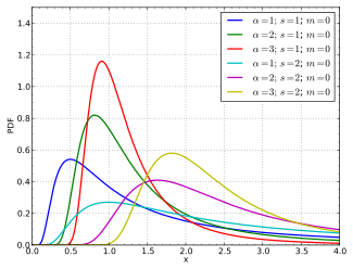
Probability density function  | |
|
Cumulative distribution function  | |
| Parameters |
 shape. shape. (Optionally, two more parameters)  scale (default: scale (default:  ) )  location of minimum (default: location of minimum (default:  ) ) |
|---|---|
| Support |
 |
 | |
| CDF |
 |
| Quantile |
![{\displaystyle \ \left[\ -\ln p\ \right]^{-{\tfrac {1}{\alpha }}}\ s+m\ }](https://wikimedia.org/api/rest_v1/media/math/render/svg/d2b5533c2d790aeca4344934fd3333e6573764fd) |
| Mean |
 |
| Median |
 |
| Mode |
 |
| Variance |
![{\displaystyle {\begin{cases}\ s^{2}\left[\ \Gamma \left(1-{\tfrac {2}{\alpha }}\right)-\left[\Gamma \left(1-{\tfrac {1}{\alpha }}\right)\right]^{2}\ \right]~~&{\text{for }}~\alpha >2\\\ \infty &{\text{otherwise}}\end{cases}}}](https://wikimedia.org/api/rest_v1/media/math/render/svg/c838d324399bc07046edc5a853425cbc6c910bd9) |
| Skewness |
 ![{\displaystyle {\begin{aligned}{\text{where}}~~A\ \equiv \ &\Gamma \left(1-{\tfrac {3}{\alpha }}\right)\\&-\ 3\ \Gamma \left(1-{\tfrac {2}{\alpha }}\right)\ \Gamma \left(1-{\tfrac {1}{\alpha }}\right)\\&\quad +\ 2{\Bigl [}\ \Gamma \left(1-{\tfrac {1}{\alpha }}\right)\ {\Bigr ]}^{3}\ \end{aligned}}}](https://wikimedia.org/api/rest_v1/media/math/render/svg/f50783e3b2ffd2c84167381d1552c31f6ae2bfad) ![{\displaystyle ~\quad {\text{and}}~~B\ \equiv \ \Gamma \left(1-{\tfrac {2}{\alpha }}\right)\ -\ {\Bigr [}\ \Gamma \left(1-{\tfrac {1}{\alpha }}\right)\ {\Bigr ]}^{2}~.}](https://wikimedia.org/api/rest_v1/media/math/render/svg/e21b3c3db74e54ccd9bd7396c72b2ea1408edded) |
| Excess kurtosis |
 ![{\displaystyle {\begin{aligned}{\text{where}}~~C\ \equiv \ &\Gamma \left(1-{\tfrac {4}{\alpha }}\right)\\&-\ 4\ \Gamma \left(1-{\tfrac {3}{\alpha }}\right)\ \Gamma \left(1-{\tfrac {1}{\alpha }}\right)\\&\qquad +\ 3\ {\Bigl [}\ \Gamma \left(1-{\tfrac {2}{\alpha }}\right)\ {\Bigr ]}^{2}\ \end{aligned}}}](https://wikimedia.org/api/rest_v1/media/math/render/svg/2b4f5d6e5baad21ca411edb4b3528bc3b66466f5) ![{\displaystyle ~\quad {\text{and}}~~D\ \equiv \ \Gamma \left(1-{\tfrac {2}{\alpha }}\right)\ -\ {\Bigl [}\ \Gamma \left(1-{\tfrac {1}{\alpha }}\right)\ {\Bigr ]}^{2}~.}](https://wikimedia.org/api/rest_v1/media/math/render/svg/4c22d44070228bd9f53fd9fdc1418db618034c63) |
| Entropy |
 where where  is the Euler–Mascheroni constant. is the Euler–Mascheroni constant. |
| MGF |
[1] Note: Moment  exists if exists if  |
| CF | [1] |
The Fréchet distribution, also known as inverse Weibull distribution,[2][3] is a special case of the generalized extreme value distribution. It has the cumulative distribution function
where α > 0 is a shape parameter. It can be generalised to include a location parameter m (the minimum) and a scale parameter s > 0 with the cumulative distribution function
Named for Maurice Fréchet who wrote a related paper in 1927,[4] further work was done by Fisher and Tippett in 1928 and by Gumbel in 1958.[5][6]
The single parameter Fréchet, with parameter 
(with 

where 
In particular:
The quantile 

.
In particular the median is:
The mode of the distribution is 
Especially for the 3-parameter Fréchet, the first quartile is ![{\displaystyle q_{1}=m+{\frac {s}{\sqrt[{\alpha }]{\log(4)}}}}](https://wikimedia.org/api/rest_v1/media/math/render/svg/72285aecb7128d3dda2842d57a231f1a2f695cef)
![{\displaystyle q_{3}=m+{\frac {s}{\sqrt[{\alpha }]{\log({\frac {4}{3}})}}}.}](https://wikimedia.org/api/rest_v1/media/math/render/svg/13ffc4910ba74fb71df3613a478b1d02ce54db63)
Also the quantiles for the mean and mode are:

- In hydrology, the Fréchet distribution is applied to extreme events such as annually maximum one-day rainfalls and river discharges.[7] The blue picture, made with CumFreq, illustrates an example of fitting the Fréchet distribution to ranked annually maximum one-day rainfalls in Oman showing also the 90% confidence belt based on the binomial distribution. The cumulative frequencies of the rainfall data are represented by plotting positions as part of the cumulative frequency analysis.
However, in most hydrological applications, the distribution fitting is via the generalized extreme value distribution as this avoids imposing the assumption that the distribution does not have a lower bound (as required by the Frechet distribution). [citation needed]

- The cumulative distribution function of the Frechet distribution solves the maximum stability postulate equation
- Scaling relations
- The Frechet distribution is a max stable distribution
- The negative of a random variable having a Frechet distribution is a min stable distribution
- ^ a b Muraleedharan, G.; Guedes Soares, C.; Lucas, Cláudia (2011). "Characteristic and moment generating functions of generalised extreme value distribution (GEV)". In Wright, Linda L. (ed.). Sea Level Rise, Coastal Engineering, Shorelines, and Tides. Nova Science Publishers. Chapter 14, pp. 269–276. ISBN 978-1-61728-655-1.
- ^ Khan, M.S.; Pasha, G.R.; Pasha, A.H. (February 2008). "Theoretical analysis of inverse Weibull distribution" (PDF). WSEAS Transactions on Mathematics. 7 (2): 30–38.
- ^ de Gusmão, Felipe R.S.; Ortega, Edwin M.M.; Cordeiro, Gauss M. (2011). "The generalized inverse Weibull distribution". Statistical Papers. 52 (3). Springer-Verlag: 591–619. doi:10.1007/s00362-009-0271-3. ISSN 0932-5026.
- ^ Fréchet, M. (1927). "Sur la loi de probabilité de l'écart maximum" [On the probability distribution of the maximum deviation]. Annales Polonici Mathematici (in French). 6: 93.
- ^ Fisher, R.A.; Tippett, L.H.C. (1928). "Limiting forms of the frequency distribution of the largest and smallest member of a sample". Proceedings of the Cambridge Philosophical Society. 24 (2): 180–190. Bibcode:1928PCPS...24..180F. doi:10.1017/S0305004100015681. S2CID 123125823.
- ^ Gumbel, E.J. (1958). Statistics of Extremes. New York, NY: Columbia University Press. OCLC 180577.
- ^ Coles, Stuart (2001). An Introduction to Statistical Modeling of Extreme Values. Springer-Verlag. ISBN 978-1-85233-459-8.
- ^ Lee, Se Yoon; Mallick, Bani (2021). "Bayesian Hierarchical Modeling: Application Towards Production Results in the Eagle Ford Shale of South Texas". Sankhya B. 84: 1–43. doi:10.1007/s13571-020-00245-8.
- Kotz, S.; Nadarajah, S. (2000). Extreme Value Distributions: Theory and applications. World Scientific. ISBN 1-86094-224-5.
- Hurairah, Ahmed; Ibrahim, Noor Akma; bin Daud, Isa; Haron, Kassim (February 2005). "An application of a new extreme value distribution to air pollution data". Management of Environmental Quality. 16 (1): 17–25. doi:10.1108/14777830510574317. ISSN 1477-7835.
- "wfrechstat: Mean and variance for the Frechet distribution". Wave Analysis for Fatigue and Oceanography (WAFO) (Matlab software & docs). Centre for Mathematical Science. Lund University / Lund Institute of Technology. Retrieved 11 November 2023 – via www.maths.lth.se.

![{\displaystyle \ \Pr(\ X\leq x\ )=\exp \left[\ -\left({\tfrac {\ x-m\ }{s}}\right)^{-\alpha }\ \right]~~{\text{ if }}~x>m~.}](https://wikimedia.org/api/rest_v1/media/math/render/svg/9d4cb73171ba319f41ff5a0d552dc9bd19371c35)


