The effect of preprocessing pipelines in subject classification and detection of abnormal resting state functional network connectivity using group ICA - PubMed
- ️Sun Jan 01 2017
Review
The effect of preprocessing pipelines in subject classification and detection of abnormal resting state functional network connectivity using group ICA
Victor M Vergara et al. Neuroimage. 2017.
Abstract
Resting state functional network connectivity (rsFNC) derived from functional magnetic resonance (fMRI) imaging is emerging as a possible biomarker to identify several brain disorders. Recently it has been pointed out that methods used to preprocess head motion variance might not fully remove all unwanted effects in the data. Proposed processing pipelines locate the treatment of head motion effects either close to the beginning or as one of the final steps. In this work, we assess several preprocessing pipelines applied in group independent component analysis (gICA) methods to study the rsFNC of the brain. The evaluation method utilizes patient/control classification performance based on linear support vector machines and leave-one-out cross validation. In addition, we explored group tests and correlation with severity measures in the patient population. We also tested the effect of removing high frequencies via filtering. Two real data cohorts were used: one consisting of 48 mTBI and one composed of 21 smokers, both with their corresponding matched controls. A simulation procedure was designed to test the classification power of each pipeline. Results show that data preprocessing can change the classification performance. In real data, regressing motion variance before gICA produced clearer group differences and stronger correlation with nicotine dependence.
Copyright © 2016 Elsevier Inc. All rights reserved.
Figures

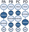
Preprocessing pipelines tested in this study. Before estimating rsFNC, a set of preprocessing steps must be applied to the raw fMRI data. The initial steps labeled as STRCoN correspond to slice-timing correction, rigid body realignment for motion, co-registration, spatial normalization, and transformation to the MNI standard space. The step labeled MotReg corresponds with removal of motion variance through regression. Step SpkReg indicates orthogonalization with respect to spike regressors. When spike and motion regressions were necessary, they were performed in one single regression step called SpkMotReg. The label Smooth-gICA indicates that smoothing and group ICA were performed. The final step on each pipeline is Filter, where a pass-band filter is applied. Four different pipelines named PA, PB, PC and PD were considered with different order of steps as displayed in this figure.

Plot used to parameterize the simulation. This shows the relationship between final Measured Correlation, Power-Ratio (PR) and correlation between artificial signals. The plot uses two different time-courses: TC1 and TC2. These time-courses were extracted from fMRI data for two different RSNs using space-time-regression. The two time courses exhibit low correlation value. Two signals, S1 and S2, are algorithmically generated to have an artificial correlation Art.Corr[S1,S2] with different values 1.0, 0.5, 0.2 and 0.1. Signals and time courses are mixed and the measured correlation corr[TC1+S1, TC2+S2] is plotted for different, PR = (var[S]/var[TC]). After 0dB, Art.Corr dominates the measured correlation, but below −12dB its influence is minimal. The simulation was performed with PR = −9dB, aiming at minimizing changes in the characteristics of original time courses TC1 and TC2, but allowing a significant correlation level of 0.2. In our data, significant correlations (p<0.05) are those surpassing the threshold of 0.16.

Spatial content of the uncorrelated RSNs used in the simulation. The mean correlation between these two RSNs was low (ideally zero) in the HC samples. Simulated connectivity was achieved using these t-maps and space time regression to extract, modify and reintroduce artificial phase information. In this figure, images were cropped using t-value thresholds between 20 and 30 and the color bars indicate these levels.

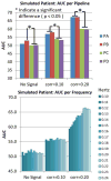
Pipeline and Frequency performances for simulated data. Simulated increments of connectivity were achieved by artificially adding time coherent signals where the correlation significance threshold (p<0.05) is 0.16. The strongest connectivity case with correlation of 0.2 demonstrates the case of a significant correlation. The case with correlation of 0.1 is an artificially simulated no-significant correlation. The baseline case show results for the case where no signal was added. Results shown are averages of either pipeline or frequency dimensions. Pipelines PA and PB exhibit better performance than PC and PD for cases where signals were introduced. Frequency results are different from chance only for the largest simulated connectivity of 0.2. The best frequency bandwidth in the 0.20 case was the range [0.01 0.22] Hz. There were no significant differences among bandwidths with high cut-off 0.20, 0.21, 0.22,0.23 and 0.24 Hz on all three bar plots. Otherwise, most of the AUC differences were significant in the frequency dimension. The number of significant differences was too high to fit in the figure.

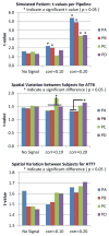
t-values and mean spatial maps deviations for simulated data. As the case of No-Signal shows, without artificial manipulation the t-value is not significant for any pipeline. However, the RSN pair in this simulation was chosen to exhibit this characteristic. The two pipelines where MotReg (or SpkMotReg which includes MotReg) was performed before gICA (see PA and PB in Figure 1) were sensitive to the artificially simulated correlation. In the pipelines where MotReg was performed after gICA (see PC and PD in Figure 1), these were only sensitive if the simulated correlation was strong enough (0.20). This figure also shows mean deviations of subject-wise spatial maps. This deviation was calculated using the Euclidean distance from the peak coordinates of the mean spatial map (averaged over all subjects) to the peak coordinates of each subject spatial map. Significantly higher deviations were detected for PC and PD in ATT6. Deviations in ATT7 were not significantly different, but a trend of higher deviation can be seen in PC and PD.

RSNs used in the analysis. This set obtained using gICA was selected based on the frequency content and visual inspection. Some RSNs in the CER group overlap with visual areas, but with a large peak region in the cerebellum and high temporal correlation with other cerebellar components. A total of 53 RSNs were identified in the mTBI sample and for all four pipelines. In the smokers sample, only 43 of these components could be matched. RSNs marked with an asterisk (*) were missing in the smokers sample. The match was confirmed by visual inspection and using a spatial correlation larger than 0.5.

Pipeline and Frequency Performance for the mTBI Sample. On each cross validation loop, the LOOCV optimization selected the pipeline and bandwidth combination with the best AUC measure. The top row displays the mean AUC performances obtained from all pipeline and bandwidth combinations applied by the LOOCV optimization. Permutation tests indicated no statistically significant differences. The bottom row shows the histograms of pipeline and bandwidth selection. Although AUC differences were not significant, the pipeline histogram follows the trend observed in AUC. PA is the most frequently selected pipeline with a higher mean AUC. Frequency bandwidths show a more uncertain distribution.

Spatial content of the significant rsFNC differences in the mTBI group. These two rsFNC are significant only in PA and PB, which are the pipelines where motion variance is removed before gICA. The t-values seemed unaffected by frequency. On the other hand, FDR corrected p-values show large variability with the bandwidth selection in PC and PD. Activation differences in the precuneus and angular gyrus areas (Olsen et al., 2014; Smits et al., 2009) suggest attentional deficits related to these areas. Abnormal rsFNC have also been found in the cerebellum (Nathan et al., 2014) and in other cases linked to post concussive complaints (Stevens et al., 2012).

Pipeline and Frequency Performance for the Smokers Sample. Differences in mean AUC are not significant for either pipelines or frequency bandwidth. The preferences for PA and high frequency bandwidth displayed by the histograms are similar to that observed in the mTBI cohort.

RSN with significant group difference corrected using FDR. In addition, this RSN pair exhibit an increase in rsFNC correlated with FTND. The spatial content of these networks suggests a resting state interaction between reward and visuospatial brain networks. The two plots on the right show changes against bandwidth selection of FTND regression coefficients and corresponding p-values for each pipeline. Although PC exhibits the largest effect size, the significance of the regression coefficient is dependent on the bandwidth. PB has the lowest effect size and also shows high instability with respect to significance. The effect sizes of PA and PD are very similar. The p-values in PA are the lowest and always significant in showing the highest level of robustness against selected bandwidth.
Similar articles
-
Depressing time: Waiting, melancholia, and the psychoanalytic practice of care.
Salisbury L, Baraitser L. Salisbury L, et al. In: Kirtsoglou E, Simpson B, editors. The Time of Anthropology: Studies of Contemporary Chronopolitics. Abingdon: Routledge; 2020. Chapter 5. In: Kirtsoglou E, Simpson B, editors. The Time of Anthropology: Studies of Contemporary Chronopolitics. Abingdon: Routledge; 2020. Chapter 5. PMID: 36137063 Free Books & Documents. Review.
-
Gautret P, Lagier JC, Parola P, Hoang VT, Meddeb L, Mailhe M, Doudier B, Courjon J, Giordanengo V, Vieira VE, Tissot Dupont H, Honoré S, Colson P, Chabrière E, La Scola B, Rolain JM, Brouqui P, Raoult D. Gautret P, et al. Int J Antimicrob Agents. 2020 Jul;56(1):105949. doi: 10.1016/j.ijantimicag.2020.105949. Epub 2020 Mar 20. Int J Antimicrob Agents. 2020. PMID: 32205204 Free PMC article. Retracted. Clinical Trial.
-
Pillay J, Gaudet LA, Saba S, Vandermeer B, Ashiq AR, Wingert A, Hartling L. Pillay J, et al. Syst Rev. 2024 Nov 26;13(1):289. doi: 10.1186/s13643-024-02681-3. Syst Rev. 2024. PMID: 39593159 Free PMC article.
-
Haeussler K, Ismaila AS, Malmenäs M, Noorduyn SG, Green N, Compton C, Thabane L, Vogelmeier CF, Halpin DMG. Haeussler K, et al. Respir Res. 2024 Dec 21;25(1):438. doi: 10.1186/s12931-024-03056-x. Respir Res. 2024. PMID: 39709425 Free PMC article. Review.
-
Interventions to reduce harm from continued tobacco use.
Lindson-Hawley N, Hartmann-Boyce J, Fanshawe TR, Begh R, Farley A, Lancaster T. Lindson-Hawley N, et al. Cochrane Database Syst Rev. 2016 Oct 13;10(10):CD005231. doi: 10.1002/14651858.CD005231.pub3. Cochrane Database Syst Rev. 2016. PMID: 27734465 Free PMC article. Review.
Cited by
-
Noro Y, Li R, Matsui T, Jimura K. Noro Y, et al. Front Neuroinform. 2023 Jan 12;16:960607. doi: 10.3389/fninf.2022.960607. eCollection 2022. Front Neuroinform. 2023. PMID: 36713290 Free PMC article.
-
An information theory framework for dynamic functional domain connectivity.
Vergara VM, Miller R, Calhoun V. Vergara VM, et al. J Neurosci Methods. 2017 Jun 1;284:103-111. doi: 10.1016/j.jneumeth.2017.04.009. Epub 2017 Apr 23. J Neurosci Methods. 2017. PMID: 28442296 Free PMC article.
-
Xie H, Calhoun VD, Gonzalez-Castillo J, Damaraju E, Miller R, Bandettini PA, Mitra S. Xie H, et al. Neuroimage. 2018 Oct 15;180(Pt B):495-504. doi: 10.1016/j.neuroimage.2017.05.050. Epub 2017 May 23. Neuroimage. 2018. PMID: 28549798 Free PMC article.
-
Chahine G, Richter A, Wolter S, Goya-Maldonado R, Gruber O. Chahine G, et al. Hum Brain Mapp. 2017 Apr;38(4):1741-1750. doi: 10.1002/hbm.23477. Epub 2016 Dec 23. Hum Brain Mapp. 2017. PMID: 28009080 Free PMC article.
-
Motion artifact in studies of functional connectivity: Characteristics and mitigation strategies.
Satterthwaite TD, Ciric R, Roalf DR, Davatzikos C, Bassett DS, Wolf DH. Satterthwaite TD, et al. Hum Brain Mapp. 2019 May;40(7):2033-2051. doi: 10.1002/hbm.23665. Epub 2017 Nov 1. Hum Brain Mapp. 2019. PMID: 29091315 Free PMC article. Review.
References
-
- Allen EA, Erhardt EB, Damaraju E, Gruner W, Segall JM, Silva RF, Havlicek M, Rachakonda S, Fries J, Kalyanam R, Michael AM, Caprihan A, Turner JA, Eichele T, Adelsheim S, Bryan AD, Bustillo J, Clark VP, Feldstein Ewing SW, Filbey F, Ford CC, Hutchison K, Jung RE, Kiehl KA, Kodituwakku P, Komesu YM, Mayer AR, Pearlson GD, Phillips JP, Sadek JR, Stevens M, Teuscher U, Thoma RJ, Calhoun VD. A baseline for the multivariate comparison of resting-state networks. Front Syst Neurosci. 2011;5:2. - PMC - PubMed
-
- Borg J, Holm L, Cassidy JD, Peloso P, Carroll L, Von Holst H, Ericson K. Diagnostic procedures in mild traumatic brain injury: results of the WHO Collaborating Centre Task Force on Mild Traumatic Brain Injury. Journal of Rehabilitation Medicine. 2004;36:61–75. - PubMed
Publication types
MeSH terms
Grants and funding
LinkOut - more resources
Full Text Sources
Other Literature Sources
Medical
Miscellaneous